Table of Contents
机器学习01-逻辑回归算法#
算法简介#
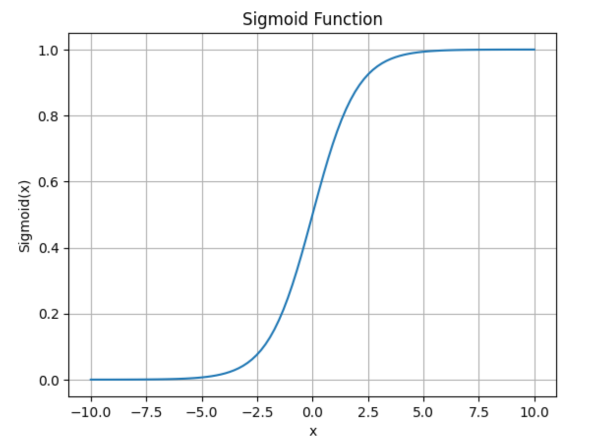
逻辑回归(Logistic Regression),是机器学习中一种十分基础的分类方法,由于算法简单而高效,在实际场景中得到了广泛的应用。假设要解决的问题是一个二分类问题,目标值为 \(\{0, 1\}\),以线性回归为基础,通过sigmoid函数将模型输出映射到 \([0, 1]\) 之间。z=0时,函数值为0.5,以0.5为分界点,将大于0.5和小于0.5的值分为两类,解决0-1二分类问题。sigmoid函数的表达式如下:
sigmoid函数图像:
推导过程#
使用sigmoid函数,逻辑回归的计算公式为:
通过 sigmoid 函数我们可以计算单个样本属于正类还是负类的概率:
我们将上面两个式子合并成一个:
有了上面这个式子,我们就能很容易的得到函数 \(h\) 在整个数据集上的似然函数:
转为对数似然函数:
假设我们用随机梯度下降法更新参数,每次只用一个样例,则上面的对数似然函数退化成:
更新参数的公式为:
这里的 \(\alpha\) 就是学习率。其次注意式子里的 “+”,因为我们要极大化对数似然函数,所以我们需要沿着梯度方向更新参数。接下来我们要做的就是求出 \(L(\theta)\) 对各个参数的偏导。
(1)首先我们知道 sigmoid 函数的求导结果为:
(2)我们可以推导出 \(L(\theta)\) 对各个参数的偏导为:
(3)所以,参数更新公式为:
(4)如果我们用梯度下降法,每次更新参数用所有样例,则参数更新公式为:
Python 实现#
数据prepare#
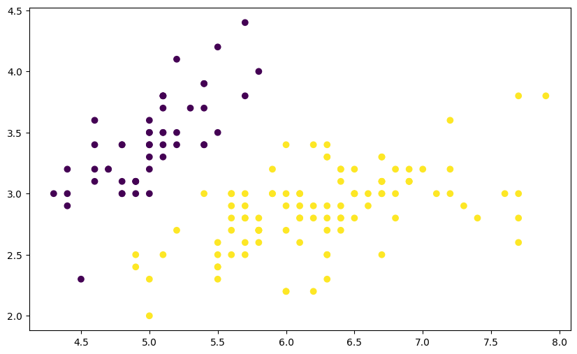
该数据集共有两个特征变量 X0 和 X1, 以及一个目标值 Y。其中,目标值 Y 只包含 0 和 1,也就是一个典型的 0-1 分类问题。我们尝试将该数据集绘制成图,看一看数据的分布情况。
import pandas as pd

df = pd.read_csv("../data/course-8-data.csv", header=0)  # 加载数据集
df.head()  # 预览前 5 行数据
| X0 | X1 | Y | |
|---|---|---|---|
| 0 | 5.1 | 3.5 | 0 |
| 1 | 4.9 | 3.0 | 0 |
| 2 | 4.7 | 3.2 | 0 |
| 3 | 4.6 | 3.1 | 0 |
| 4 | 5.0 | 3.6 | 0 |
from matplotlib import pyplot as plt
%matplotlib inline

plt.figure(figsize=(10, 6))
plt.scatter(df['X0'], df['X1'], c=df['Y'])
<matplotlib.collections.PathCollection at 0x119e08ac0>
算法实现#
数据分为两类,接下来,就运用逻辑回归完成对两类数据的划分。
import numpy as np


def sigmoid(z):
    """sigmoid函数"""
    sigmoid = 1 / (1 + np.exp(-z))
    return sigmoid


def loss(h, y):
    """损失函数"""
    loss = (-y * np.log(h) - (1 - y) * np.log(1 - h)).mean()
    return loss


def gradient(X, h, y):
    """计算梯度"""
    gradient = np.dot(X.T, (h - y)) / y.shape[0]
    return gradient


def Logistic_Regression(x, y, lr, num_iter):
    """逻辑回归过程(y=wx+b)"""
    # 初始化截距为 1
    intercept = np.ones((x.shape[0], 1))

    x = np.concatenate((intercept, x), axis=1)
    w = np.zeros(x.shape[1])   # 初始化参数为 0

    for i in range(num_iter):  # 梯度下降迭代
        z = np.dot(x, w)       # 线性函数
        h = sigmoid(z)         # sigmoid 函数
        g = gradient(x, h, y)  # 计算梯度
        w -= lr * g            # 通过学习率 lr 计算步长并执行梯度下降
        l = loss(h, y)         # 计算损失函数值

    return l, w                # 返回迭代后的梯度和参数
x = df[['X0', 'X1']].values
y = df['Y'].values
lr = 0.01         # 学习率
num_iter = 30000  # 迭代次数

# 训练
L = Logistic_Regression(x, y, lr, num_iter)
L
(0.05103697443193302, array([-1.47673791, 4.27250311, -6.9234085 ]))
结果展示#
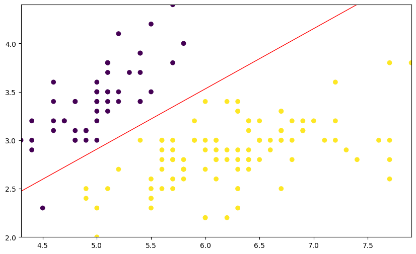
有了分类边界线函数,我们就可以将其绘制到原图中,看一看分类的效果到底如何。下面这段绘图代码涉及到 Matplotlib 绘制轮廓线,不需要掌握。
plt.figure(figsize=(10, 6))
plt.scatter(df['X0'], df['X1'], c=df['Y'])

x1_min, x1_max = df['X0'].min(), df['X0'].max(),
x2_min, x2_max = df['X1'].min(), df['X1'].max(),

xx1, xx2 = np.meshgrid(np.linspace(x1_min, x1_max),
                       np.linspace(x2_min, x2_max))

grid = np.c_[xx1.ravel(), xx2.ravel()]

probs = (np.dot(grid, np.array([L[1][1:3]]).T) + L[1][0]).reshape(xx1.shape)
plt.contour(xx1, xx2, probs, levels=[0], linewidths=1, colors='red')
<matplotlib.contour.QuadContourSet at 0x119ec1d00>
scikit-learn实现#
prepare数据#
import pandas as pd

df = pd.read_csv("../data/course-8-data.csv", header=0)  # 加载数据集
x = df[['X0', 'X1']].values
y = df['Y'].values
算法实现#
from sklearn.linear_model import LogisticRegression

model = LogisticRegression(tol=0.001, max_iter=10000, solver='liblinear')  # 设置数据解算精度和迭代次数
model.fit(x, y)
model.coef_, model.intercept_
(array([[ 2.49579289, -4.01011301]]), array([-0.81713932]))
model.score(x, y)
0.9933333333333333
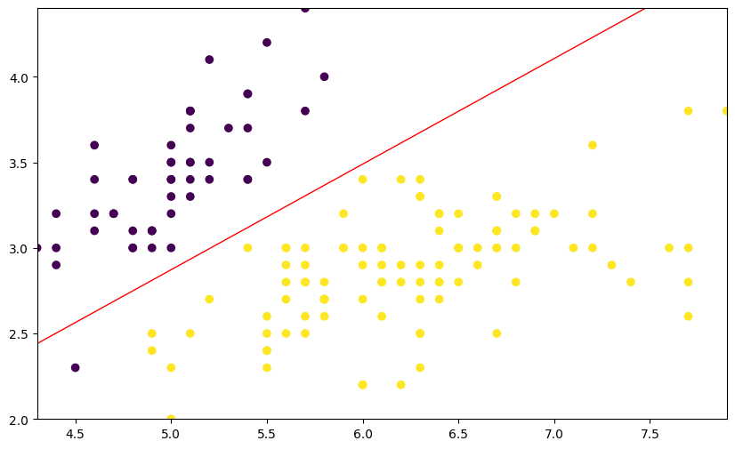
结果展示#
import numpy as np
from matplotlib import pyplot as plt
%matplotlib inline

plt.figure(figsize=(10, 6))
plt.scatter(df["X0"], df["X1"], c=df["Y"])

x1_min, x1_max = df["X0"].min(), df["X0"].max()
x2_min, x2_max = df["X1"].min(), df["X1"].max()

xx1, xx2 = np.meshgrid(np.linspace(x1_min, x1_max), np.linspace(x2_min, x2_max))
grid = np.c_[xx1.ravel(), xx2.ravel()]

probs = (np.dot(grid, model.coef_.T) + model.intercept_).reshape(xx1.shape)
plt.contour(xx1, xx2, probs, levels=[0], linewidths=1, colors="red")
<matplotlib.contour.QuadContourSet at 0x1035321c0>